Tutorial 1: Optimization¶

This tutorial is a step-by-step walk through of simulation-based optimization. This tutorial builds on the tutorial in Section Tutorial 2: Creating a Flowsheet with Linked Simulations.

The files for this tutorial are located in: examples/test_files/Optimization/Model_Files

Note

The examples/ directory refers to the location where the FOQUS examples were installed, as described in Install FOQUS Examples.

Open FOQUS.
Load the FOQUS session from the tutorial “Creating a Flowsheet with Linked Simulations” in Section Tutorial 2: Creating a Flowsheet with Linked Simulations or if that tutorial has not yet been completed, complete it first.

Problem Set Up¶

If the simulation runs successfully and the results are reasonable, proceed to define the optimization problem. There are four steps to setting up the optimization problem: (1) select the variables, (2) define samples (optional), (3) define the objective function, and constraints and (4) select and configure the solver.

Select the Optimization button from the toolbar at the top of the Home window (Figure Optimization Problem Variables). Select the Variables tab.
Select “Decision” from the drop-down list in the Type column as the variable type for all 17 variables shown. If more than 17 variables are shown, the edge connecting the “BFB” node to the “Cost” node was most likely not configured properly. The scale will automatically change to linear, which is acceptable for most problems.
The Min, Max, and Value columns can be changed. The Min and Max columns define the lower and upper bounds. The Value column specifies the initial point. For this example the defaults are acceptable.

If more than one flowsheet evaluation is used in the objective function calculation (e.g., parameter estimation or optimization under uncertainty), the next step is to setup the samples under the Samples tab. In this case only one evaluation is used to calculate an objective function value, so the sample setup is not needed. 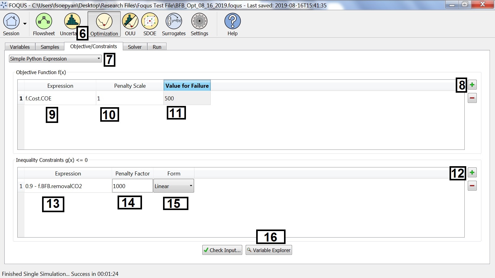The next step is to define the objective function and constraints using the form under the Objective/Constraints tab as shown in Figure Optimization Problem Objective.

Select the Objective/Constraints tab (see Figure Optimization Problem Objective).
In the drop-down list, verify “Simple Python Expression” is selected.
Add an objective function by clicking + to the right of the Objective Function table.
The objective function is the cost of electricity from the cost spreadsheet. Enter:

f.Cost.COE

in the Expression column.
Enter 1 in the Penalty Scale column. This setting is used mostly for multi-objective optimization to apply the constraint penalty to different objectives.
Enter 500 in the Value for Failure column. This should be worse than the objective for any non-failed simulations.
Add a constraint by clicking + next to the Inequality Constraints table.
The constraint is that the fraction of CO\(_2\) captured must be greater than or equal to 0.9. The constraint is in the form \(g(\mathbf{x}) \leq 0\); therefore, in the Expression column enter:

0.9 - f.BFB.removalCO2.
Enter 1000 for the Penalty Factor.
The constraint penalty Form should be linear.
The Variable Explorer button can be used to help select flowsheet variables.

Solver Settings¶

The last step before running the optimization is to select and configure the solver. The solver configuration form is shown in Figure Optimization Solver Setup.

Select the Solver tab (see Figure Optimization Solver Setup).
Select “OptCMA” from the Select Solver drop-down list.
The default options are acceptable. Solver options are described in the Solver Options table.

Running Optimization¶

The optimization run form is shown in Figure Optimization Monitor.

Click the Run tab to display the optimization run form (see Figure Optimization Monitor).
Click Start.
Once the optimization has run for while click Stop.

As the optimization run, the best result found is stored in the Flowsheet. If an optimization is run with sample variables the first sample in the set with the best objective function will be stored in the flowsheet. All simulation results can be viewed in the Flowsheet Results table.

The run form displays some diagnostic information as the optimization runs. The parts of the display labeled in Figure Optimization Monitor are described below.

The Optimization Solver Messages window displays information from the solver.
The Best Solution Parallel Coordinate Plot shows the value of the scaled decision variables, which is useful to see where the best solution is relative to the variable bounds.
The Objective Function Plot shows the best value of the objective function found as a function of the optimization iteration or sample number.
While the optimization is running, the status bar shows the amount of time that has elapsed since starting the optimization.