Tutorial 2: Parameter Estimation
Note: The NLopt solvers are used for the tutorial, but are an optional to the installation. See the install instructions for more information about installing NLopt.
This tutorial provides a very simple example of using the sampling with optimization. Sampling can be used to do optimization under uncertainty where there are several scenarios with differing values of uncertain parameters. Sampling can also be used to do parameter estimation, where estimated values must be compared against several data points. This tutorial will focus on parameter estimation.
At any point in this tutorial, the FOQUS session can be saved and the tutorial can be started again from that point.
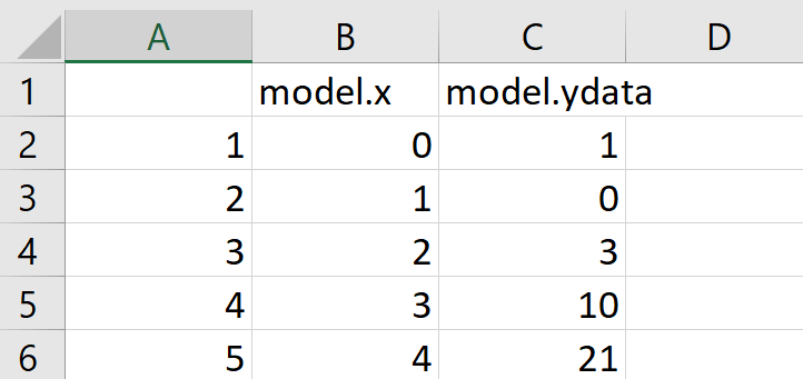
The model is given by Equation (1). The unknown parameters are \(a\), \(b\), and \(c\). The x and y data are given in Table x-y Data.
Sample |
1 |
2 |
3 |
4 |
5 |
|---|---|---|---|---|---|
x |
0 |
1 |
2 |
3 |
4 |
y |
1 |
0 |
3 |
10 |
21 |
The first step is to create a flowsheet with one node. The node will have the input variables: a, b, c, x, and ydata; and output variable y.
Open FOQUS.
In the Session Name field, enter “PE_tutorial” (see Figure Session Setup).
Click the Flowsheet button in the top toolbar.

Session Setup
Add a node to the flowsheet named “model.”
Click Add Node in the left toolbar (see Figure Adding Node and Inputs).
Click anywhere on the gridded flowsheet area.
Select “model” in the Name drop-down list and then click OK.
Click the Selection Mode icon in the left toolbar (see Figure Adding Node and Inputs).
Click the Node Editor icon in the left toolbar (see Figure Adding Node and Inputs).
In the Node Edit input table, add the variables a, b, c, x, and ydata. The ydata variable will be used as an input for the known y sample point data, later in the tutorial.
Click the Add Input icon (see Figure Adding Node and Inputs).
Enter “a” for the variable name in the Name column.
Enter -10 and 10 for the min and max in the Min and Max columns for a, b, c, and x.
Repeat for all of the inputs.
Enter 1 for the value of a, b, and c in the Value column.
Enter 2 for the value of x in the Value column.
The Value, Min, and Max for ydata do not matter.
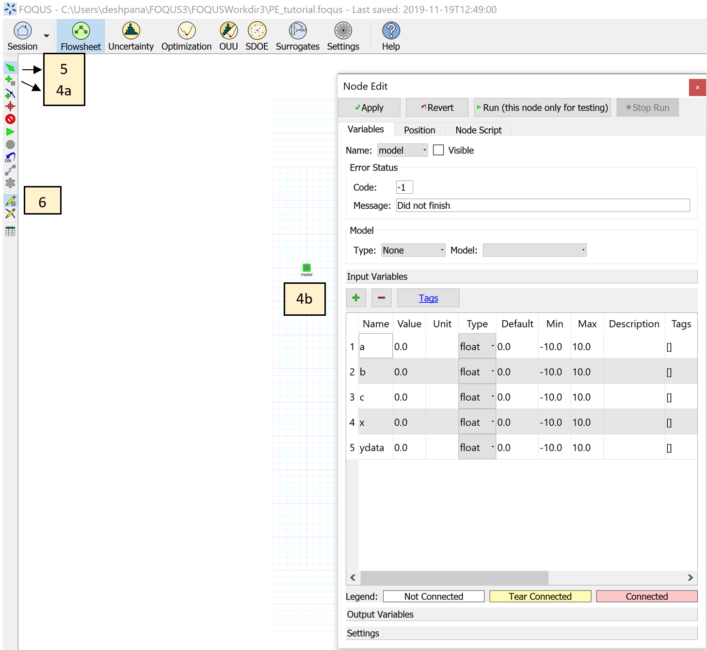
Adding Node and Inputs
Click Output Variables (see Figure Adding Outputs).
Add the output variable y.
Click the Add Output icon (see Figure Adding Outputs).
Enter “y” for the variable name in the Name column.

Adding Outputs
Add the model equation to the node.
Click the Node Script tab.
Enter the following code in the calculations box:
f['y'] = x['a']*x['x']**2\
 + x['b']*x['x'] + x['c']

Adding Node Calculation
Return to the Output Variables table in the Node Editor, by clicking on the Variables tab, and selecting Output Variables.
Click Run in the left toolbar in the FOQUS Home window, to test a single flowsheet evaluation and ensure there are no errors.
When the run is complete, there should be no error and the value of y should be 7 in the Output Variables table.
The next step is to setup the optimization. The objective function is to minimize the sum of the squared errors between the estimated value of y and the observed value of y. There are five data points in Table x-y Data, so there are five flowsheet evaluations that need to go into the calculation of the objective.
Click the Optimization button in the top toolbar of the Home window (see Figure Optimization Variables).
- Select “Decision” in the Type column drop-down lists for “model.a,” “model.b,” and“model.c.” The Scale column will automatically be set to linear.
Select “Sample” in the Type column drop-down lists for “model.x” and “model.ydata.”

Optimization Variables
The decision variables in the optimization problem will be changed by the optimization solver to try to minimize the objective, and the sample variables are used to construct the samples that will go into the objective function calculation.
Select the Samples tab (see Figure Optimization Samples).
Click Add Sample five times to add five samples.
Enter the data from Table x-y Data in the Samples table.
For larger sample sets, Generate Samples has an option to load from a CSV file. The CSV file must be saved as “CSV (MS-DOS)” as the file type, as follows:
Sample Variable data (csv file)

Optimization Samples
The objective function is the sum of the square difference between y and ydata for each sample in Table x-y Data. The optimization solver changes the a, b, and c to minimize the objective.
Click the Objective/Constraints tab.
Click the Add Objective icon on the right side of the Objective Function table (see Figure Objective Function).
In the Expression column, enter the following (without any line break):
sum([(ff.model.y - xx.model.ydata)**2 for (ff,xx) in zip(f,x)])
The above expression uses Python list comprehension to calculate the sum of squared errors.
- The keys for x (the inputs) and f (the outputs) are:
Dummy variable name for index (i.e., ff for outputs and xx for inputs)
Node name (i.e., model)
Variable name (i.e., y and ydata)
Then, the user will need to specify which of the dummy index corresponds to outputs, and which of the dummy index corresponds to inputs. In this case, ff is for the outputs, and xx is for the inputs. Hence, we have “for (ff,xx) in zip(f,x)” (without the quotes).
Enter 1 for the Penalty Scale.
Enter 100 for the Value for Failure.
No constraints are required.
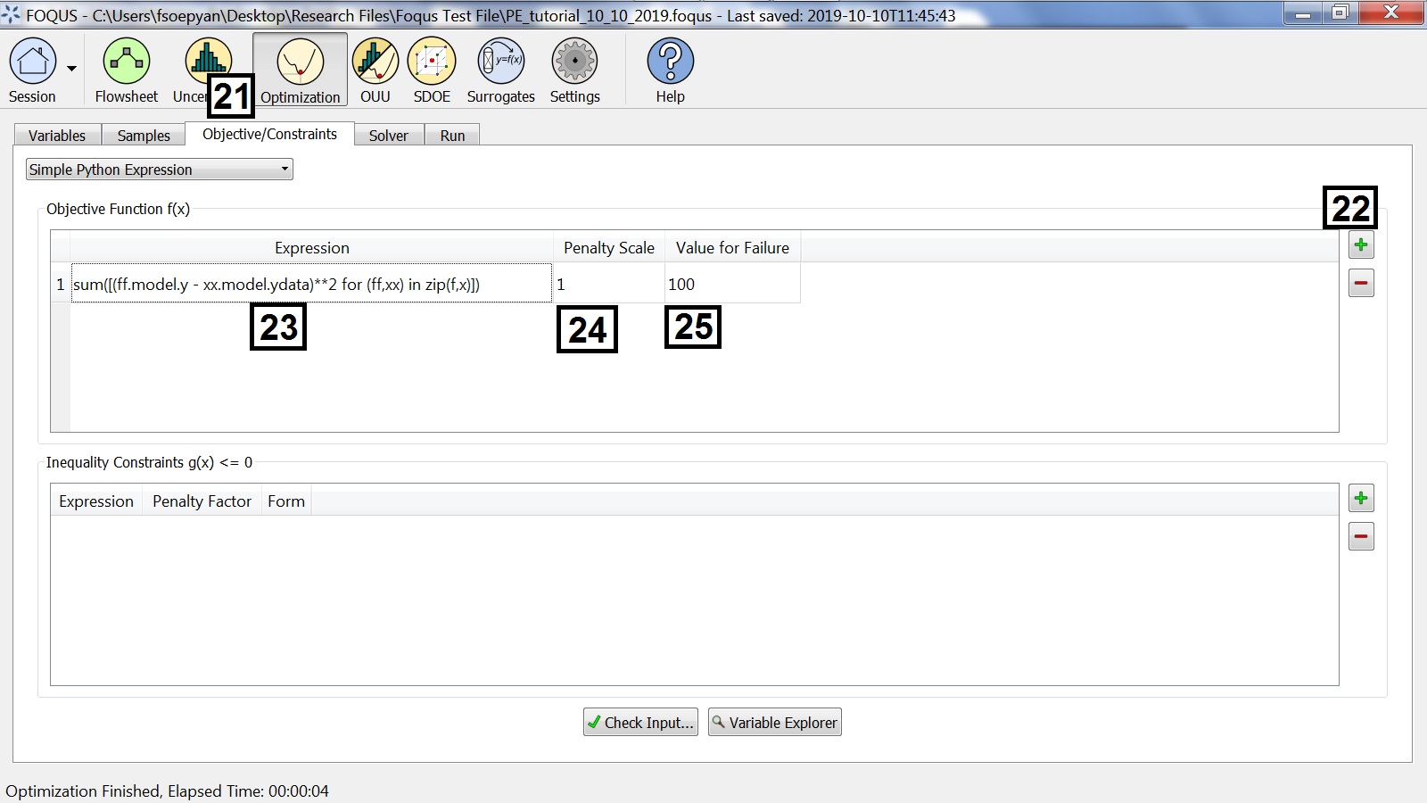
Objective Function
Once the objective is set up, a solver needs to be selected and configured. Almost any solver in FOQUS should work well for this problem with the default values.
Click the Solver tab (see Figure Optimization Samples).
Select “NLopt” from the Select Solver drop-down list. NLopt is a collection of solvers that share a standard interface (Johnson 2015).
Select “BOBYQA” under the Solver Options table in the Settings column drop-down list.

Optimization Samples
Click the Run tab (see Figure Running Optimization).
Click the Start button.
The Optimization Solver Messages window displays the solver progress. As the solver runs, the best results found is placed into the flowsheet.
The Best Solution Parallel Coordinate Plot shows the scaled decision variable values for the best solution found so far.
The Objective Function Plot shows the value of the objective function as the optimization progresses.

Running Optimization
The best result at the end of the optimization is stored in the flowsheet. All flowsheet evaluations run during the optimization are stored in the flowsheet results table.
Once the optimization has completed, click Flowsheet in the top toolbar.
Open the Node Editor and look at the Input Variables table. The approximate result should be \(a = 2\), \(b = -3\), and \(c = 1\) (see Figure Flowsheet, Input Variables Results).

Flowsheet, Input Variables Results