Example USF-1: Constructing Uniform Space Filling minimax and maximin designs for a 2-D input space
For this first example, the goal is to construct a simple space-filling design with between 8 and 10 runs in a 2-dimensional space based on a regular unconstrained square region populated with a grid of candidate points.
From the FOQUS main screen, click the SDOE button. On the top left side, select Load Existing Set, and select the SDOE_Ex1_Candidates.csv file from examples folder. This identifies the possible input combinations from which the design will be constructed. The more possible candidates that can be provided to the search algorithm used to construct the design, the better the design might be for the specified criterion.
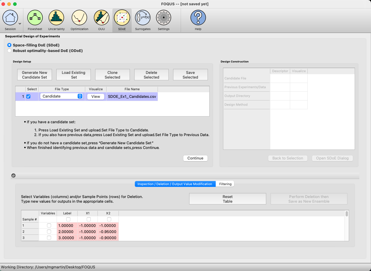
Ex 1 Design Setup
Next, by selecting View and then Plot it is possible to see the grid of points that will be used as the candidate points. In this case, the range for each of the inputs, X1 and X2, has been chosen to be between -1 and 1.
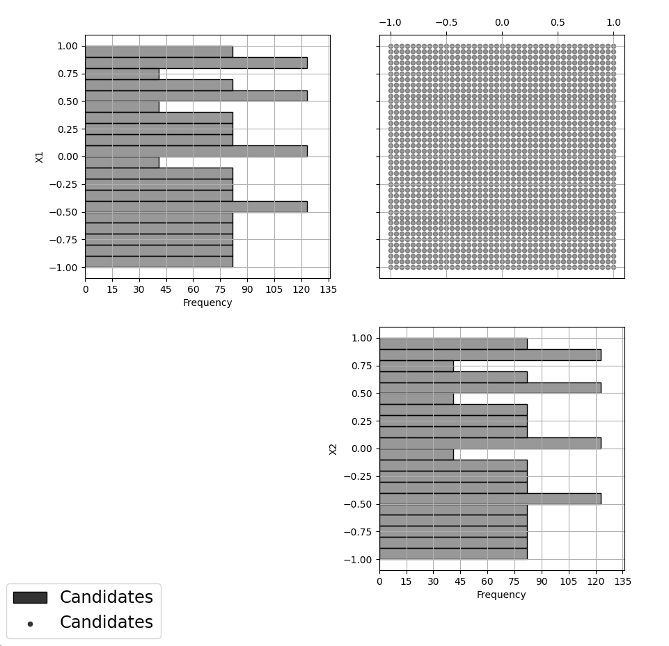
Ex 1 Candidate Grid
Next, click on Continue to advance to the Design Construction Window, and then select Uniform Space Filling and click on Open SDoE Dialog to advance to the second SDOE screen, where particular choices about the design can be made. On the second screen, select minimax for the Optimality Method Selection. Change the Min Design Size and Max Design Size to 8 and 10, respectively. This will construct 3 minimax designs of size 8, 9 and 10. Next, uncheck the column called Label. This will mean that the design is not constructed using this as an input. There should be an _id column automatically created containing unique identifiers to identify which runs from the candidate set were chosen for the final designs. Since the ranges of each of X1 and X2 are the bounds that we want to use for creating this design, we do not need to change the entries in Min and Max.
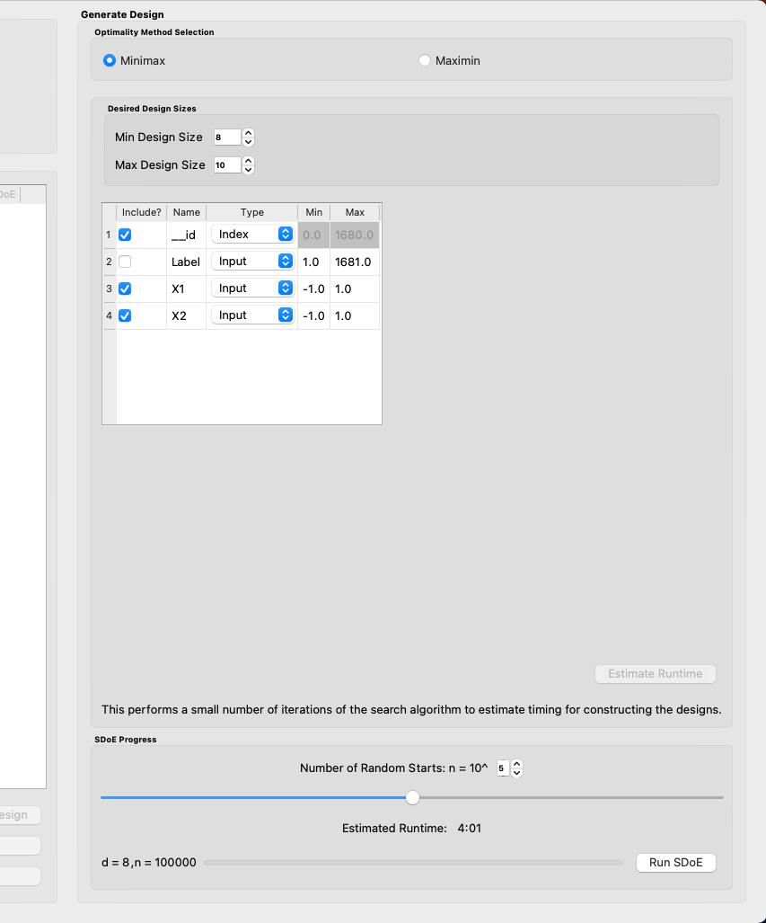
Ex 1 Minimax design choices
Once the choices for the design have been specified, click on the Estimate Runtime button to estimate the time taken for creating the designs. For the computer on which this example was developed, if we ran the minimum number of random starts (10^3=1000), it is estimated that the code would take 2 seconds to create the three designs (of size 8, 9 and 10). If we chose 10^4=10000 runs, then the code is estimated to take 24 seconds. It is estimated that 10^5=100000 random starts would take 4 minutes and 1 second, while 10^6=1 million random starts would take approximately 41 minutes and 29 seconds. In this case, we selected to create designs based on 100000 random starts, since this was a suitable balance between timeliness and giving the algorithm a chance to find the best possible designs. Hence, select 10^5 for the Number of Random Starts, and then click Run SDOE.
Since we are also interested in examining maximin designs for the same scenario, we click on the Go Back to Generate Design button in the Created Designs window to repopulate the right window with the same choices that we made for all of the design options.
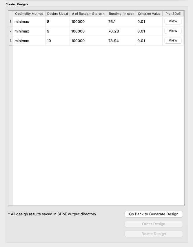
Ex 1 Minimax created designs
After changing the Optimality Method Selection to maximin, click on Estimate Runtime, select 10^5 for the Number of Random Starts, and then click Run SDOE. After waiting for the prescribed time, the Created Designs window will have 6 created designs - three that are minimax designs and three that are maximin designs.
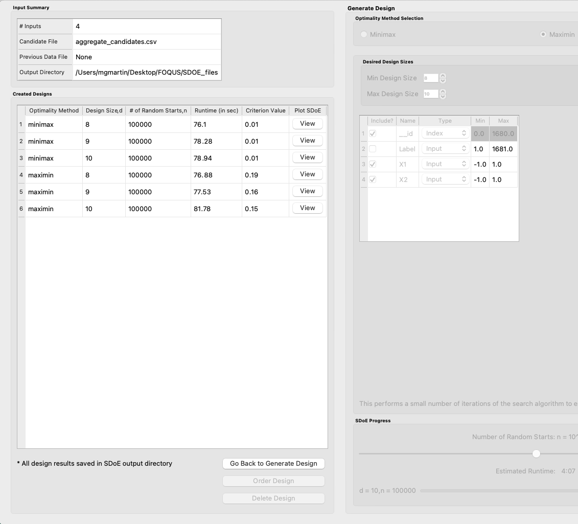
Ex 1 Created designs
We now consider the choices between the designs to determine which is the best match for our experimental goals. We can see a list of the selected design points by clicking View for any of the created designs, and Plot allows us to see the spread of the design points throughout the input region.
Clearly, there is a trade-off between the cost of the experiment (larger number of runs involve more time, effort and expense) and how well the designs fill the space. When choosing which of the designs is most appropriate for the experiment, it is important to remember that resources spent early in the process cannot be used later, so it is helpful to balance early learning about the process, with the ability to identify and focus on the desired optimal location later.
There is also a small difference in priorities between the minimax and the maximin criteria. Minimax seeks to minimize how far any candidate point (which defines our region of interest) is from a design point. Maximin seeks to spread out the design points and maximize how close the nearest points are to each other. As noted previously, minimax designs tend to avoid putting too many points on the edge of the region, while maximin designs often place a number of points right on the edges of the input space.
By looking at the placement of the points, how well they fill the desired space, and the points proximity to the edge of the region, the user can find a good match for their experimental goals. After considering all of the trade-offs between the alternatives, select the design that best matches the goals of the experiment.
The file for the selected design can be found in the SDOE_files folder. The design can then be used to guide the implementation of the experiment with the input factor levels for each run.
Example USF-2: Augmenting the Example USF-1 design in a 2-D input space with a Uniform Space Filling Design
In this example, we consider the sequential aspect of design, by building on the first example results. Consider the scenario where based on the results of Example 1, the experimenter selected to actually implement and run the 8 run minimax design.
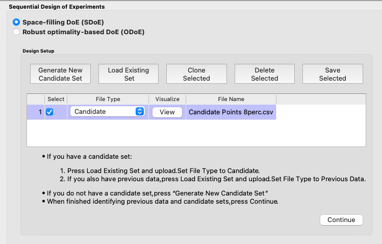
In the Design Setup box, click on Load Existing Set to select the candidate set that you would like to use for the construction of the design. This may be the same candidate set that was used in Example 1, or it might have been updated based on what was learned from the first data collection. For example, if it was learned that one corner of the design space might not be desirable, then the candidate set can be updated to remove candidate points that are now considered undesirable. For the File Type leave the designation as Candidate.
To load in the experimental runs that were already collected, click on Load Existing Set again, and select the design file that was created in the SDOE_files folder. This time, change the File Type to Previous Data. If you wish to view either of the candidate or previous data files, click on View to see either a table or plot.
Click on the Continue button at the bottom right of the Design Setup box. This will activate the Design Construction box.
After examining that the desired files have been selected, click on the Uniform Space Filling button at the bottom right corner of the Design Construction window. This will open the second SDOE window that shows the Sequential Design of Experiments Set-Up window on the right hand side.
Select Minimax or Maximin for the type of design to create.
Select the Min Design Size and Max Design Size to match what is desired. If you wish to just generate a single design of the desired size, make Min Design Size = Max Design Size. Recall that this will be the number of additional points that will be added to the existing design, not the total design size.
Next, select the options desired in the box: a) Should any of the columns be excluded from the design creation? If yes, then unclick the Include? box. b) For input factors to be used in the construction of the uniform space filling design, make sure that the Type is designated as Input. The automatically generated index column __id will be already listed as Index. If there is a label column for the candidates, then uncheck its Include? box to make sure only one index column is used. c) Finally, you can optionally change the Min and Max ranges for the inputs to adjust the relative emphasis that distances in each input range are designated.
Once the set-up choices have been made, click Estimate Runtime to find out what the anticipated time is for generating designs based on different numbers of random starts.
Select the number of random starts to use, based on available time. Recall that using more random starts is likely to produce a design that is closer to the overall best optimum.
After the SDOE module has created the design(s), the left window Created Designs is populated with the new design(s). These can be viewed with the View option, where the plot now shows the Previous Data in pink, and the newly added possible design in blue. This allows better assessment of the appropriateness of the new design subject to the data that have already been collected.
To access the file that contains the created designs, go to the SDOE_files folder. As before, a separate folder will have been created for each design.
If there is a desire to do another set in the sequential design, then the procedure outlined above for Example 2 can be followed again. The only change will be that this time there will be 3 files that need to be imported: A Candidate file from which new runs can be selected, and two Previous Data files. The first of these files will be the selected design from Example USF-1, and the second the newly created design that was run as a result of Example USF-2. When the user clicks on Continue in the Design Setup window, the two Previous Data files will be aggregated into a single Aggregated Previous Data file.
Example USF-3: A Uniform Space Filling Design for a Carbon Capture example in a 5-D input space
In this example, we consider a more realistic scenario of a sequential design of experiment. Here we explore a 5-dimensional input space with G, lldg, CapturePerc, L and SteamFlow denoting the space that we wish to explore with a space-filling design. The candidate set, Candidate Points 8perc, contains 93 combinations of inputs that have been validated using an ASPEN model as possible combinations for this scenario. The goal is to collect 18 runs in two stages that fill the input space. There are some constraints on the inputs, that make the viable region irregular, and hence the candidate set is useful to avoid regions where it would be problematic to collect data.
After selecting the SDOE tab in FOQUS, click on Load Existing Set and select the candidate file, Candidate Points 8perc.
Ex 3 Design Setup window
To see the range of each input and how the viable region of interest is captured with the candidate set, select View and then plot. In this case we have chosen to just show the 5 input factors in the pairwise scatterplot.
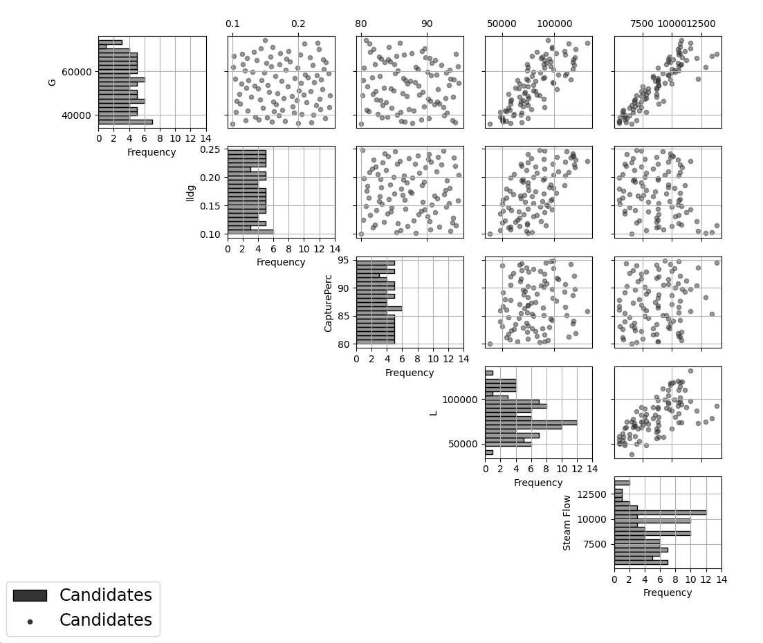
Ex 3 plot of viable input space as defined by candidate set
After clicking Continue in the Design Setup box, and then Uniform Space Filling from the Design Construction box, the Generate Design box will appear on the right side of the second window. Here, select the options desired for the experiment to be run. For the illustrated figure, we selected a Minimax design with 3 potential sizes: 10, 11, 12. We specified that the column __id will be used as the Index, G, lldg, CapturePerc, L, SteamFlow will define the 5 factors to be used as inputs. We unclicked the Include? box for CO2 captured since we do not want to use it in the design construction, and also unclicked the Include? box for Test No. as we already have an index column with __id.
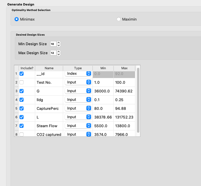
Ex 3 generate design window for first stage
After clicking Estimate Runtime and selecting the number of random starts to be used, click Run SDOE. After the module has created the requested designs, they can be viewed and compared.

Ex 3 10,11,12 run designs created for first stage
By clicking View and then Plot, the designs can be viewed. Suppose that the experimenter decides to use the 12 run design in the initial phase, then this would be the design that would be implemented and data collected for these 12 input combinations.
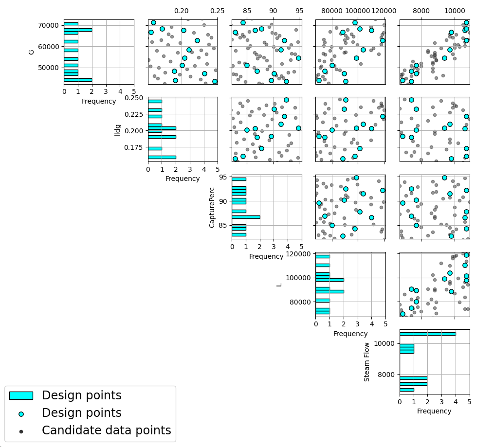
Ex 3 chosen experiment for first stage
After these runs have been collected, the experimenter wants to collect additional runs. In this case, return to the first SDOE module window, and load in the candidate set (which can be changed to reflect any knowledge gained during the first phase, such as undesirable regions or new combinations to include). The completed experiment should also be included as a Previous Data file, by going to the SDOE_files folder and selecting the file containing the appropriate design. Note that all candidate file(s) and previous data file(s) used together must contain all the same column names, with the exception of the __id column since it is automatically created later on.
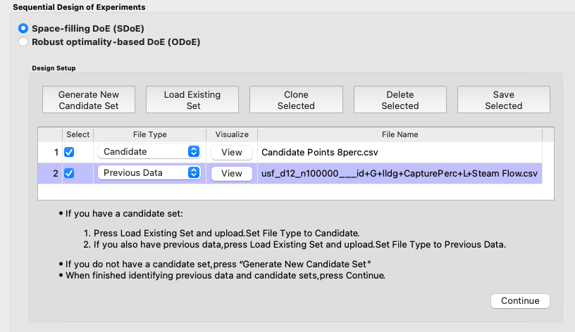
Ex 3 design setup box for second stage
After clicking Continue in the Design Setup box, and then Uniform Space Filling from the Design Construction box, the Generate Design box will appear on the right side of the second window. Here, select the options desired for the experiment to be run. For the illustrated figure, we selected a Minimax design with a design size of 6 (to use the remaining available budget). We again specified that the column __id will be used as the Index, G, lldg, CapturePerc, L, SteamFlow will define the same 5 factors to be used as inputs, and we uncheck the unneeded columns Test No. and CO2 captured.
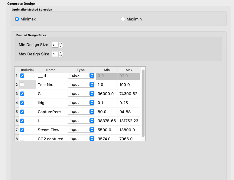
Ex 3 generate design box for second stage
After clicking Estimate Runtime and selecting the number of random starts to be used, click Run SDOE. After the module has created the requested design, it can be viewed. After selecting View and then Plot, the experimenter can see the new design with the previous data runs included. This provides a good plot to allow the complete sequence of two experiments to be examined as a combined set of runs. Note that the first and second stages are shown in different colors. The first stage is shown in pink while the second is shown in blue. Candidate points not part of either stage are in gray.
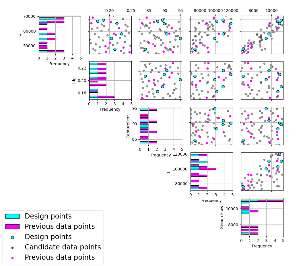
Ex 3 chosen experiment for second stage