Basic Steps for a Uniform Space Design
We now consider some details for each of these steps:
1. In the Design Setup box, click on the Load Existing Set button to select the file(s) for the construction of the design. Several files can be selected and added to the box listing the chosen files.
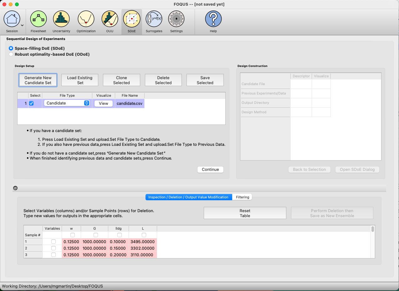
SDOE Home Screen
2. For each of the files selected using the pull-down menu, identify them as either a Candidate file or a Previous Data file. Candidate .csv files are comprised of possible input combinations from which the design can be constructed. The columns of the file should contain the different input factors that define the dimensions of the input space. The rows of the file each identify one combination of input values that could be selected as a run in the final design. Typically, a good candidate file will have many different candidate runs listed, and they should fill the available design region to be considered. Leaving gaps or holes in the input space is possible, but generally should correspond to a region where it is not possible (or desirable) to collect data. The flexibility of the candidate set approach allows for linear and non-linear constraints for one or more of the inputs to be incorporated easily.
Previous Data .csv files should have the same number of columns for the input space as the candidate file (with matching column names), and represent data that have already been collected. The algorithm for creating the design aims to place points separated from where data have already been obtained, while filling the input space around those locations. If the experiment is being run sequentially, the Previous Data file should use the input values that were actually implemented, not the target values from the previous designed experiment.
Both the Candidate and Previous Data files should be .csv files that have the first row as the Column heading. The Input columns should be numeric. Additional columns are allowed and can be identified as not necessary to the design creation at a later stage.
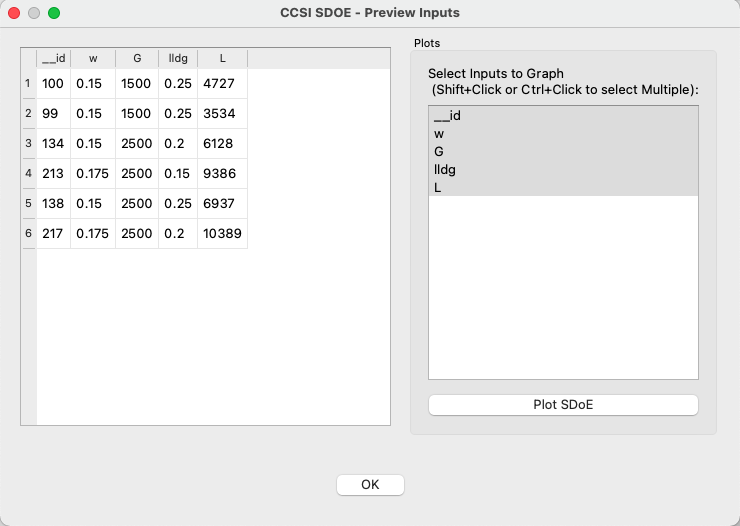
3. Click on the View button to open the Preview Inputs pop-up widow, to see the list of columns contained in each file. The left hand side displays the first few rows of input combinations from the file. Select the columns that you wish to see graphically in the right hand box , and then click on Plot SDOE to see a scatterplot matrix of the data.
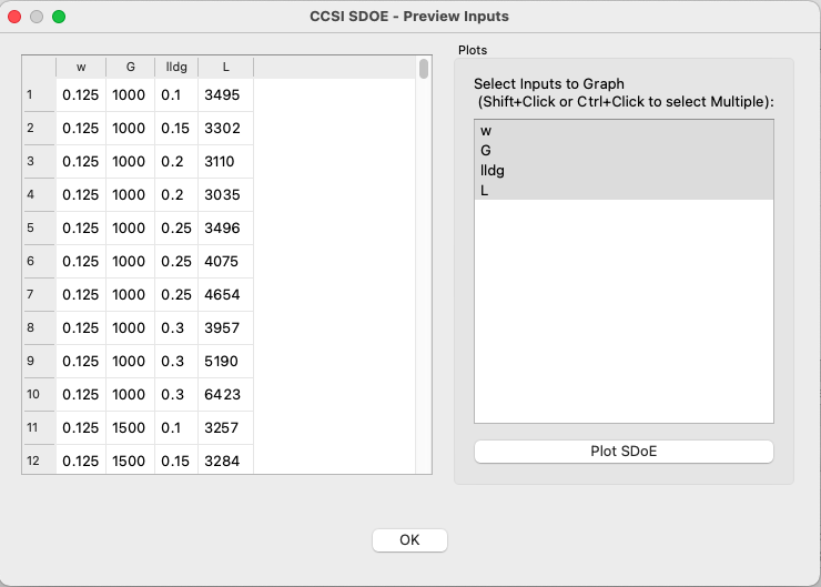
SDOE view candidate set inputs
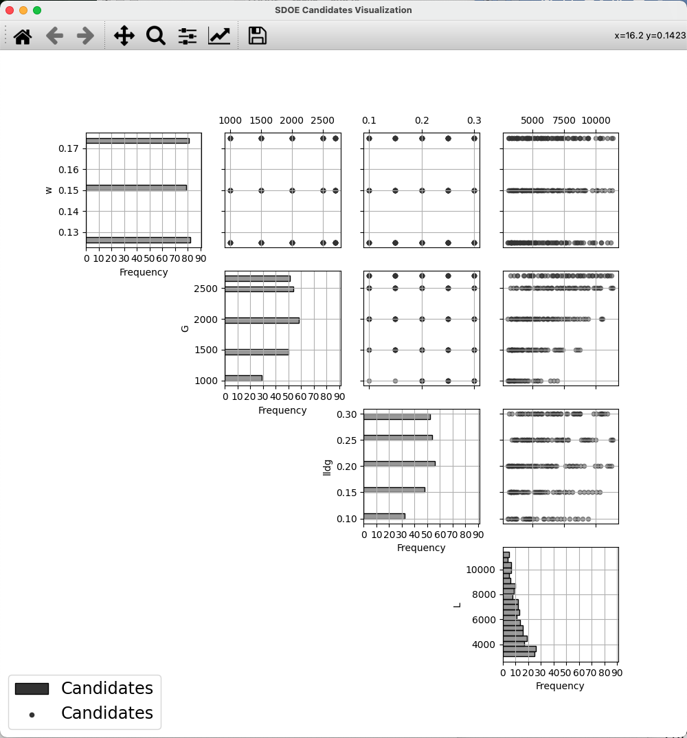
SDOE plot of candidate set inputs
The plot shows histograms of each of the inputs on the diagonals to provide a view of the distribution of values as well as the range of each input. The off-diagonals show pairwise scatterplots of each pair of inputs. This should provide the experimenter with the ability to assess if the ranges specified and any constraints for the inputs have been appropriately captured by the specified candidate set. In addition, repeating this process for any previous data will provide verification that the already observed data have been suitably summarized. Candidate set values are shown in gray, while previous data, if provided, is shown in pink.
4. Once the data have been verified for both the Candidate and Previous Data files (if a Previous Data file has been included), click on the Continue button to make the Design Construction window active.
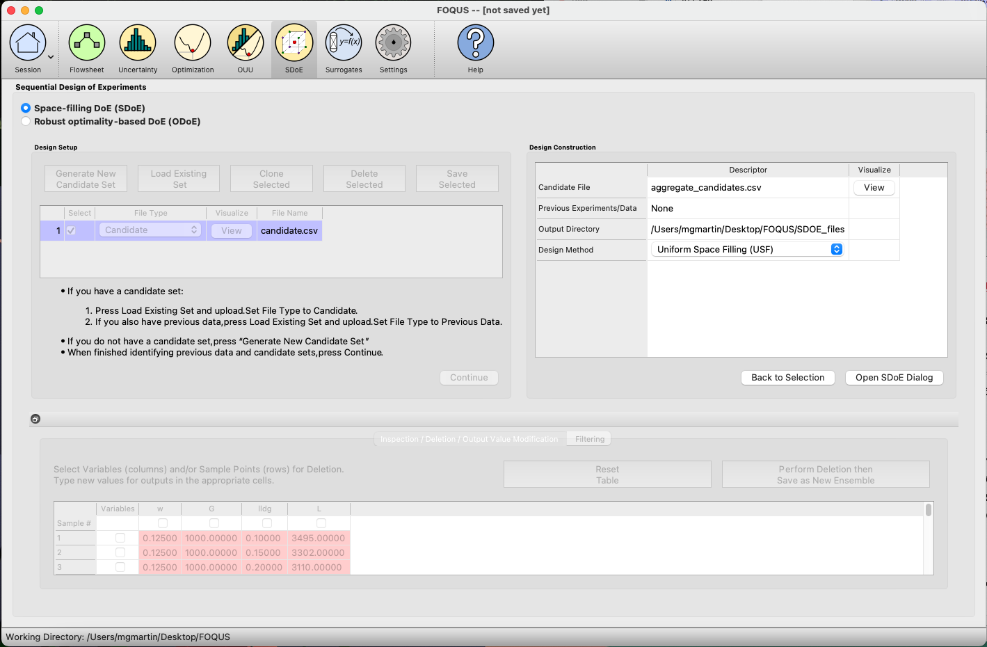
SDOE Design Construction
5. If more than one Candidate file was specified, then the aggregate_candidates.csv file that was created will have combined these files into a single file. Similarly if more than one Previous Data file was specified, then the aggregate_previousData.csv file will have been created with all runs from all these files. If only a single file was selected for either the Candidate and Previous Data files, then their corresponding aggregated files will be the same as the original.
Note
There are options to view the aggregated files for both the candidate and previous data files, simply scroll to the right of the Design Construction window, with a similar interface as was shown in step 3. In addition, a single plot of the combined candidate and previous data files can be viewed. In this plot the points representing the candidate locations and points of already collected data from the previous data file are shown in different colors.
6. Once the data have been verified as the desired set to be used for the design construction, then click on the Uniform Space Filling button at the bottom right corner of the Design Construction window, then select Open SDoE Dialog. This opens the second SDoE window, which allows for specific design choices to be made.
SDOE second window
7. The first choice to be made for the design is whether to optimize using minimax or maximin. The first choice, minimax, looks to choose design points that minimize the maximum distance that any point in the input space (as characterized by the candidate set and previous data, if it is available) is away from a design point. Hence, the idea here is that if we want to use data to help predict new outcomes throughout the input space, then we never want to be too far away from a location where data was observed.
The second choice, maximin looks to choose a design where the design points are as far away from each other as possible. In this case, the design criterion is looking to maximize how close any point is from their nearest neighbor. In practice the two design criterion often give similar designs, with the maximin criterion tending to push the chosen design points closer to the edges of the specified regions.
Hint
If there is uncertainty about some of the edge points in the candidate set being viable options, then minimax would be preferred. If the goal is to place points throughout the input space with them going right to the edges, then maximin would be preferred. Note, that creating the designs is relatively easy, so we recommend trying both approaches to examine them and then choose which is preferred based on the summary plots that are provide later.
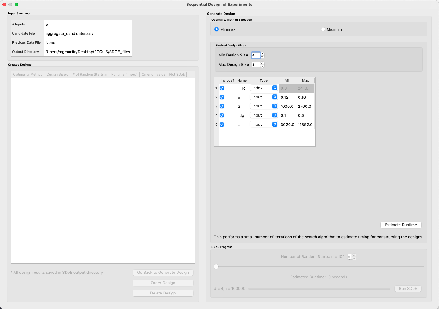
8. The next choice falls under Desired Design Size, where the experimenter can select the sizes of designs to be created. The Min Design Size specifies the smallest design size to be created. Note that the default value is set at 2, which would lead to choosing the best two design runs from the candidate set to fill the space (after taking into account any previous data that have already been gathered).
The Max Design Size specifies the largest design size to be created. The default value is set at 8, which means that if this combination were used, designs would be created of size 2, 3, 4, 5, 6, 7 and 8. The number of integers between Min Design Size and Max Design Size determines the total number of searches that the SDoE algorithm will perform. Hence, it is prudent to make a thoughtful choice for this range, that balances design sizes that are potentially of interest with the waiting time for the designs to be created. In the figure above, the Min Design Size has been changed to 4, so that only the designs of size 4, 5, 6, 7 and 8 will be created.
9. Next, there are options for the columns of the candidate set to be used for the construction of the design. Under Include? in the box on the right hand side, the experimenter has the option of whether particular columns should be included in the space-filling design search. Unclick a box, if a particular column should not be included in the space filling criterion search.
Next select the Type for each column. Typically most of the columns will be designated as Inputs, which means that they will be used to construct the best uniform space filling design. In addition, we recommend including one Index column which contains a unique identifier for each run of the candidate set. This makes it easier to track which runs are included in the constructed designs. If no Index column is specified, a warning appears later in the process, but this column is not strictly required.
Notice there is a new variable included in the first row of this box called __id. This column is an automatically-generated index of all rows of the candidate set, meaning the column counts up from 1, uniquely identifying each row. For example, if the candidate set contains 50 rows excluding the row of column names, the __id column would be 1, 2, 3, …, 49, 50. The Include box next to __id can be unchecked if including this index column is not desired, but again, it is highly encouraged to have an index column to easily identify which candidate set rows are chosen in the design. The __id column Type is automatically set to Index. If using a different variable as the index column, make sure to uncheck the Include box next to __id and also change the Type of the desired index column to Index.
Finally, the Min and Max columns in the box allow the range of values for each input column to be specified. The default is to extract the smallest and largest values from the candidate and previous data files, and use these as the Min and Max values, respectively. This approach generally works well, as it scales the inputs to be in a uniform hypercube for comparing distances between the design points.
Hint
The default values for Min and Max can generally be left at their defaults unless: (1) the range of some inputs represent very different amounts of change in the process. For example, if temperature is held nearly constant, while a flow rate changes substantially, then it may be desirable to extend the range of the temperature beyond its nominal values to make the amount of change in temperature more commensurate with the amount of change in the flow rate. This is a helpful strategy to make the calculated Euclidean distance between any points a more accurate reflection of how much of an adjustment each input requires. (2) if changes are made in the candidate or previous data files. For example, if one set of designs are created from one candidate set, and then another set of designs are created from a different candidate set. These designs and the achieved criterion value will not be comparable unless the range of each input has been fixed at matching values.
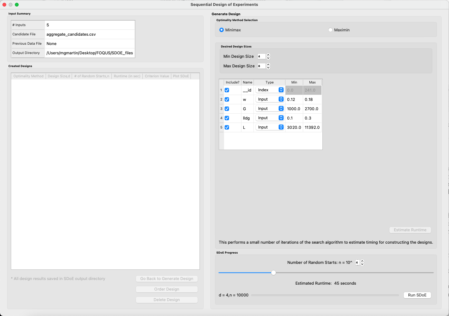
10. Once the design choices have been made, click on the Estimate Runtime button. This performs a small number of iterations of the search algorithm to calibrate the timing for constructing and evaluating the designs. The time taken to generate a design is a function of the size of the candidate set, the size of the design, as well as the dimension of the input space. The slider below Estimate Runtime now indicates an estimate of the time to construct all of the designs across the range of the Min Design Size and Max Design Size specified. The smallest Number of Random Starts is 10^3 = 1000, and is generally too small to produce a good design, but this will run very quickly and so might be useful for a demonstration. However, it would generally be unwise to use a design generated from this small a set of random starts for an actual experiment. Powers of 10 can be chosen with an Estimated Runtime provided below the slider.
SDOE second window after clicking Estimate Runtime
Hint
The choice of Number of Random Starts involves a trade-off between the quality of the design generated and the time spent waiting to generate the design. The larger the chosen number of random starts, the better the design is likely to be. However, there are diminishing gains for increasingly large numbers of random starts. If running the actual experiment is expensive, it is generally recommended to choose as large a number of random starts as possible for the available time frame, to maximize the quality of the constructed design.
11. Once the slider has been set to the desired Number of Random Starts, click on the Run SDOE button, and initiate the construction of the designs. The progress bar indicates how design construction is advancing through the chosen range of designs between the specified Min Design Size and Max Design Size values.
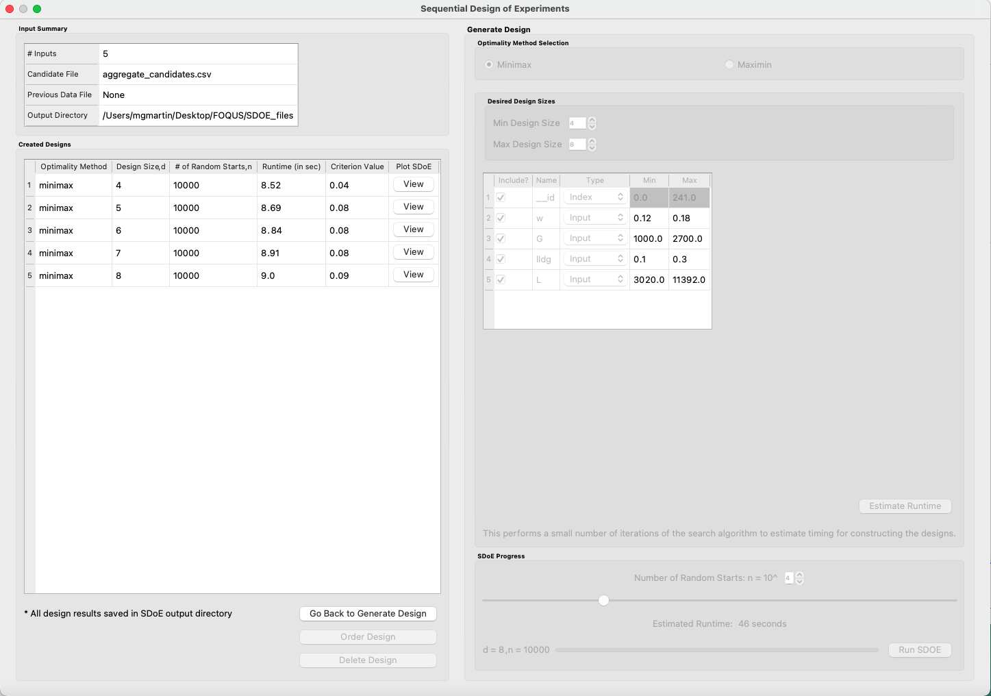
12. When the SDOE module has completed the design creation process, the left window Created Designs will be populated with files containing the results. The column entries summarize the key features of each of the designs, including Optimality Method (whether minimax or maximin was selected), Design Size (d, the number of runs in the created design), # of Random Starts, Runtime (number of seconds needed to create the design), Criterion Value (the value obtained for the minimax or maximin criterion for the saved design).
SDOE Created Designs
13. To see details of the design, the View button at the right hand side of each design row can be selected to show a table of the design, as well as a pairwise scatterplot of any subset of the input columns for the chosen design. The table and plot of the design are similar in characteristics to their counterparts described above for the candidate set. Candidate points and previous data are still shown in gray and pink, respectively, while the newly selected design points are shown in blue.
SDOE table of created design
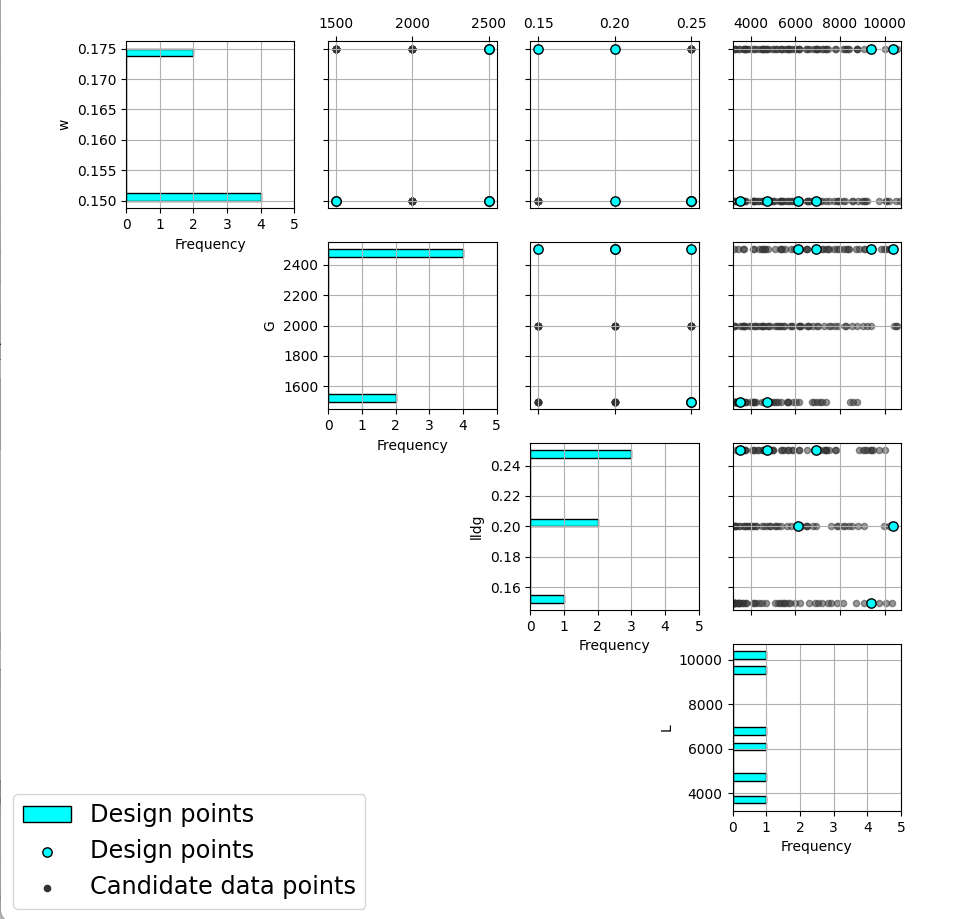
SDOE pairwise plot of created design
14. To access the file with the generated design, go to the SDOE_files folder, and a separate folder will have been created for each of the designs. In the example shown, 5 folders were created for the designs of size 4, 5, 6, 7 and 8, respectively. In each folder, there is a file containing the design, with a name that summarizes some of the key information about the design. For example, candidates_d6_n10000_w+G+lldg+L contains the design created using the candidate set called candidates.csv, with d=6 runs, based on n=10000 random starts, and based on the 4 inputs W, G, lldg and L.
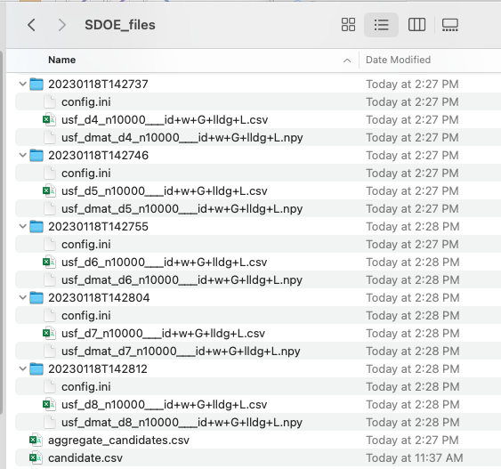
SDOE directory
When one of the design files is opened it contains the details of each of the runs in the design, with the input factor levels that should be selected for that run. If an index column was included in the design, the index value will also be shown.
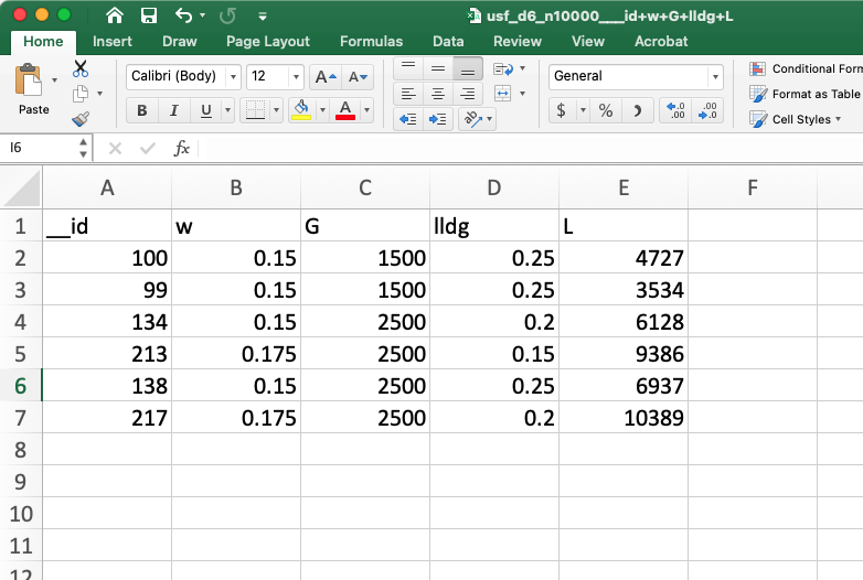
SDOE file containing a created design
To evaluate the designs that have been created, it is helpful to look at a number of summaries, including the criteria values and visualizing the spread of the design points throughout the region. Recall that at the beginning of the design creation process we recommended constructing multiple designs, with different design sizes. By examining multiple designs, it is easier to determine which design is best suited to the requirements of the experiment.
In the Created Designs table, it is possible to see the criterion values for each of the designs. For minimax designs, the goal is to minimize how far away any point in the candidate set is away from a design point. Hence, smaller values of this criterion are better. It should be the case, that a larger design size will result in smaller values, as there are more design points to distribute throughout the input space, and hence any location should have a design point closer to it. When evaluating between different sizes of design, it is helpful to think whether the improvement in the design criterion justifies the additional budget from a larger design.
For maximin designs, the goal is to maximize the distance between nearest neighbors for all design points. So for designs of the same size, we want the distance between neighboring points to be as large as possible, as this means that we have achieved near equal spacing of the design points. However, when we are comparing designs of different sizes, then the maximin criterion can be a bit confusing. Adding more runs to the design will mean that nearest neighbors will need to get closer together, and hence we would expect that on average the criterion value would get smaller for larger experiments. As with the minimax designs, we want to evaluate whether the closer packing of the design points from a larger experiment is worth the increase in cost for the additional runs.
Hint
Note that the criterion values for minimax and maximin should not be compared - one is comparing distances between design points and the candidate points, while the other is comparing distances between different design points.
For all of the designs, it is important to use the View option to look at scatterplots of the chosen design. When Previous Data points have been incorporated into the design, the plots will show how the overall collection of points fills the input space. When examining the scatterplots, it is important to assess (a) how close the design points have been placed to the edges of the region?, (b) are there holes in the design space that are unacceptably large?, and (c) does a larger design show a worthwhile improvement in the density of points to justify the additional expense?
Based on the comparison of the criterion values and the visualization of the spread of the points, the best design can be chosen that balances design performance with an appropriate use of the available budget. Recall that with sequential design of experiments, runs that are not used in the early stages might provide the opportunity for more runs at later stages. So the entire sequence of experimental runs should be considered when making choices about each stage.