[sec:ouu_overview]

Reference

The FOQUS OUU module supports several variants of optimization under uncertainty. This chapter first presents the mathematical formulations of these variants. Subsequently, details of the OUU graphical user interface will be discussed.

OUU Variables

Suppose a simulation model is available for an OUU study. Let this simulation model be represented by the following function:

\[ \begin{align}\begin{aligned}Y = F(Z_1,Z_2,Z_3,Z_4),\\which is characterized by four types of variables:\end{aligned}\end{align} \]

1. Design/Decision/Optimization variables
   • Notation: \(Z_1\) with dimension \(n_1\)
   • Definition: Design variables are continuous variables that may be bounded or unbounded. They are generally the set of optimization variables in a single-stage optimization or the set of outer optimization variables in the two-stage optimization.
2. Recourse/Operating variables
   • Notation: \(Z_2\) with dimension \(n_2\)
   • Definition: Operating variables are optimization variables in the inner optimization for a given scenario (or realization) of the uncertain variables in a two-stage optimization.
3. Discrete uncertain variables
   • Notation: \(Z_3\) with dimension \(n_3\)
   • Definition: Discrete variables are uncertain variables that have an enumerable set of states (called scenarios) such that each state is associated with a finite probability and the sum of probabilities for all the scenarios is equal to \(1\).
4. Continuous uncertain variables
   • Notation: \(Z_4\) with dimension \(n_4\)
   • Definition: Continuous uncertain variables are associated with a joint probability distribution function from which a sample can be drawn to compute the basic statistics.

OUU Objective Functions

In the presence of uncertainties, OUU seeks to find the optimal solution in some statistical sense. For example, an optimization goal may to be find the design settings that minimizes the statistical mean of the system response. Other popular objective functions are:

1. a linear combination of statistical mean and standard deviation of some selected output,
2. probability of exceeding the best value is smaller than some percentage at any point in the design space (this is analogous to conditional value at risk).

Note that these metrics are defined in the design variable space - that is, at each iteration of an OUU algorithm, the selected metric will be computed for the decision point under consideration. Since the calculation of these statistical metrics requires a sample (possibly large), OUU can benefit from parallel computing capabilities (e.g., the Turbine gateway).

Mathematical Formulations

FOQUS supports two types of OUU methods: single-stage OUU and two-stage OUU. The main difference between single-stage and two-stage OUU is the presence of the recourse (or operational) variables. Strictly speaking, since recourse variables are generally hidden (they are only needed in the inner stage and their values are not used in the outer stage of two-stage OUU), the distinction between single-stage and two-stage OUU is not clear. Nevertheless, for the sake of clarify, we will describe details of each formulation separately. The current OUU does not support linearly or nonlinearly-constrained optimization.

Single-Stage Formulation

In this formulation, there is no recourse variable:

\[ \begin{align}\begin{aligned}Y = F(Z_1, Z_3, Z_4)\\and the optimization problem becomes:\end{aligned}\end{align} \]

\[\min_{Z_1} \mathbf{\Phi}_{Z_3,Z_4} \left[ F(Z_1,Z_3,Z_4) \right]\]

where \(\Phi_{Z_3,Z_4} [F(Z_1,Z_3,Z_4)]\) is the statistical metric (one of the three options given above).

For example, if the objective function is the statistical mean, then the formulation becomes:

\[\min_{Z_1} \mathbf{E}_{Z_3,Z_4} [F(Z_1,Z_3,Z_4)] \approx \min_{Z_1} { \sum^{n_3}_{j=1} \pi_j \left( \int {F(Z_1,Z_3,Z_4) P(Z_4) d Z_4} \right)}\]

where, again, \(n_3\) is the number of scenarios for the discrete uncertain variables, \(\pi_j\) is the probability of the \(j\)-th scenario, and \(P(Z_4)\) is the joint probability of the continuous uncertain variables.

Two-Stage Formulation

In this formulation all four types of variables are present. The objective function is given by:

\[\begin{array}{lcl} & & \displaystyle \min_{Z_3,Z_4} \mathbf{\Phi}_{Z_3,Z_4} \left[ \min_{Z_2} F(Z_1,Z_2,Z_3,Z_4) \right]. \end{array}\]

If the objective function is the statistical mean, the formulation becomes:

\[ \begin{align}\begin{aligned}\begin{split} \begin{array}{lcl} & & \displaystyle \min_{Z_1} \mathbf{E}_{Z_3,Z_4} \left[ \min_{Z_2} F(Z_1,Z_2,Z_3,Z_4) \right]\\ &\approx& \displaystyle \min_{Z_1} \sum^{n_3}_{j=1} \pi_j \left( \int \left[ \min_{Z_2} F(Z_1,Z_2,Z_3,Z_4) \right] P(Z_4) d Z_4 \right) \end{array}\end{split}\\Let\end{aligned}\end{align} \]

\[ \begin{align}\begin{aligned}G(\mathbf{Z_1,Z_3,Z_4}) = \min_{Z_2} F(Z_1,Z_2,Z_3,Z_4).\\Then the two-stage equation can be rewritten as:\end{aligned}\end{align} \]

\[ \begin{align}\begin{aligned}\begin{split} \begin{array}{lcl} & & \displaystyle \min_{Z_1} \mathbf{E}_{Z_3,Z_4} \left[ G(Z_1,Z_3,Z_4) \right]\\ &\approx& \displaystyle \min_{Z_1} \sum^{n_3}_{j=1} \pi_j \left( \int G(Z_1,Z_3,Z_4) P(Z_4) d Z_4 \right) \end{array}\end{split}\\which is a single-stage OUU with respect to the :math:`G` function.\end{aligned}\end{align} \]

Windows Users

Before using the OUU module, Windows users may need to update the following registry keys:

1. HKEY_CLASSES_ROOT\Applications\python.exe\shell\open\command
2. HKEY_CLASSES_ROOT\py_auto_file\shell\open\command

To update these registry keys:

1. Open the Registry Editor by going to the Windows Start menu, typing “regedit” (without the quotes), and selecting “regedit” (Figure regedit in the Windows Start menu).

regedit in the Windows Start menu

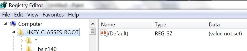
2. After the Registry Editor is opened, locate “HKEY_CLASSES_ROOT” (Figure HKEY_CLASSES_ROOT in the Registry Editor).

HKEY_CLASSES_ROOT in the Registry Editor

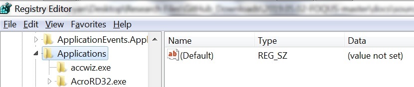
3. Under “HKEY_CLASSES_ROOT”, locate “Applications” (Figure Applications under HKEY_CLASSES_ROOT).

Applications under HKEY_CLASSES_ROOT

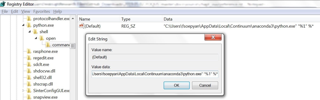
4. Under “Applications”, locate “python.exe\shell\open\command” (Figure python under Applications).

python under Applications

5. In the table on the right, double-click “(Default)” under “Name” (Figure python under Applications).
6. In the input box (Figure python under Applications), type (including the quotations): “the location of the Anaconda 3 version of python.exe” “%1” %*
7. After clicking “OK”, the information you typed in the input box should appear under “Data” in the table on the right (Figure python under Applications).
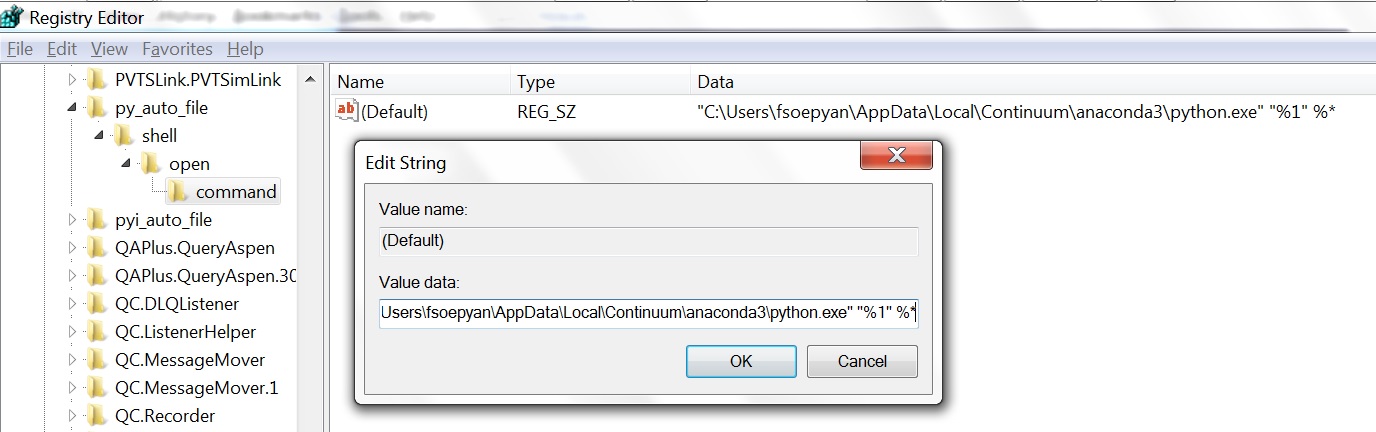
8. Under “HKEY_CLASSES_ROOT”, locate “py_auto_file\shell\open\command” (Figure py_auto_file under HKEY_CLASSES_ROOT).

py_auto_file under HKEY_CLASSES_ROOT

9. In the table on the right, double-click “(Default)” under “Name” (Figure py_auto_file under HKEY_CLASSES_ROOT).
10. In the input box (Figure py_auto_file under HKEY_CLASSES_ROOT), type (including the quotations): “the location of the Anaconda 3 version of python.exe” “%1” %*
11. Note that the code in Step 10 and Step 6 are the same (Figure python under Applications).
12. After clicking “OK”, the information you typed in the input box should appear under “Data” in the table on the right (Figure py_auto_file under HKEY_CLASSES_ROOT).

OUU User Interface

The OUU module enables the user to perform optimization under uncertainty studies on a flowsheet. From the OUU tab, the user can set up the different types of optimization parameters, select from the different OUU options, and run the optimization. This screen is shown in Figure [fig:ouu_screen].

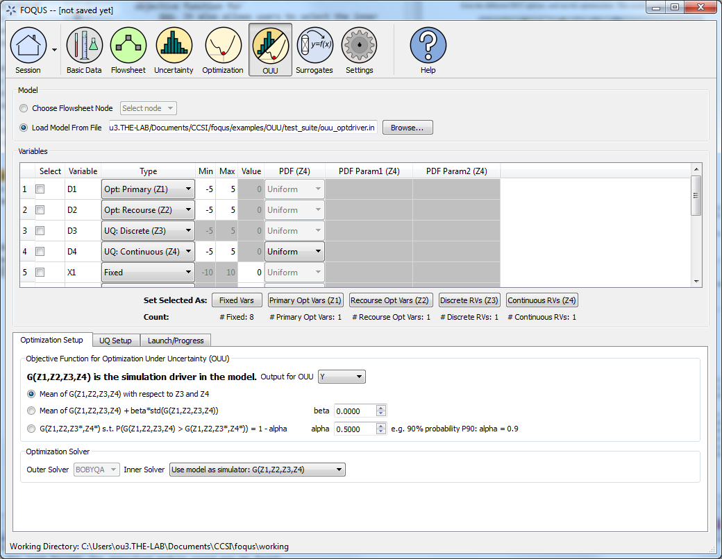
Optimization Under Uncertainty Screen

1. Model provides two options for setting up the model: (1) select a node from the flowsheet that has already been instantiated; or (2) load the model from a file in the PSUADE full file format (with the opt_driver variable set to the simulation executable.)
2. Variables displays all variables defined in the model that can be used in this context. Each available variable can be set to either one of the 6 types:
   • “Fixed”: The parameter’s value is fixed throughout the optimization process.
   • “Opt: Primary Continuous (Z1)”: Continuous parameter for the outer optimization.
   • “Opt: Primary Discrete (Z1d)”: Discrete parameter for the outer optimization.
   • “Opt: Recourse (Z2)”: Recourse parameter for the inner optimization.
   • “UQ: Discrete (Z3)”: Discrete or categorical uncertain parameter that contributes to scenarios.
   • “UQ: Continuous (Z4)”: Continuous uncertain parameter with a given probability distribution.
3. Optimization Setup allows users to select the objective function for OUU. It also allows users to select the inner optimization solver. There are two options for the inner solver: (1) the simulation model provided by users is an optimizer itself, and (2) the simulation provided by users needs to be wrapped around by another optimizer in FOQUS.
4. UQ Setup allows users to set up the continuous uncertain parameters. There are two options: (1) FOQUS can generate a sample internally, or (2) a user-generated sample can be loaded into FOQUS. The sample size should be larger than the number of continuous uncertain parameters. Optionally, response surface can be turned on to enable the statistical moments to be computed more accurately even with small samples. Users can also select a smaller subset of the sample for building response surfaces and evaluate the response surfaces with the larger samples.
5. Launch/Progress has the ‘Run OUU’ button to launch OUU runs.