MATLAB-FOQUS interface - tutorials
Problem Statement: Steady-State Continuous Stirred Tank Reactor (CSTR)
This example solves a non-linear system of equations which describes a mathematical model for a Continuous Stirred Tank Reactor (CSTR) at steady state. The CSTR is cooled with a cooling coil, and a simple exothermic reaction takes place inside the reactor (see Figure 1). Model main assumptions: 1) the reactant is perfectly mixed, and 2) the volume, heat capacities and densities are constants. Further details regarding the model are given in Vojtesek and Dostal, 2011.
Source: Jiri Vojtesek and Petr Dostal. Use of MATLAB Environment for Simulation and Control of CSTR. International Journal of Mathematics and Computers in Simulation, 6(5), 2011.

Figure 1 - Representation of a CSTR with exothermic reaction
The CSTR model in steady-state is represented by the following non-linear system of equations, which was obtained from mass and energy balances of the reactant and cooling.
where \(\mathrm{a_{1-4}}\) are constants calculated as follows:
The fixed parameters of the system are given below.
| Parameter | Symbol [Unit] | Value |
|---|---|---|
| Reactor’s volume | \(\mathrm{V\:[l]}\) | 100 |
| Reaction rate constant | \(\mathrm{k_{0}\:[min^{-1}]}\) | 7.2e10 |
| Activation energy divided by R | \(\mathrm{E/R\:[K]}\) | 1e4 |
| Reactant’s feed temperature | \(\mathrm{T_{0}\:[K]}\) | 350 |
| Inlet coolant temperature | \(\mathrm{T_{c0}\:[K]}\) | 350 |
| Reaction heat | \(\mathrm{\Delta H\:[cal\cdot mol^{-1}]}\) | -2e5 |
| Specific heat of the reactant | \(\mathrm{c_{p}\:[cal\cdot g^{-1}\cdot K^{-1}]}\) | 1 |
| Specific heat of the cooling | \(\mathrm{c_{pc}\:[cal\cdot g^{-1}\cdot K^{-1}]}\) | 1 |
| Density of the reactant | \(\mathrm{\rho\:[g\cdot l^{-1}]}\) | 1e3 |
| Density of the cooling | \(\mathrm{\rho_{c}\:[g\cdot l^{-1}]}\) | 1e3 |
| Feed concentration | \(\mathrm{c_{A0}\:[mol\cdot l^{-1}]}\) | 1 |
| Heat transfer coefficient | \(\mathrm{h_{a}\:[cal\cdot min^{-1}\cdot K^{-1}]}\) | 7e5 |
| Volumetric flow rate of reactant | \(\mathrm{q_{0}\:[l\cdot min^{-1}]}\) | 100 |
| Volumetric flow rate of cooling | \(\mathrm{q_{c0}\:[l\cdot min^{-1}]}\) | 80 |
The variables in the system of equations are described below:
| Variable | Symbol [Unit] |
|---|---|
| Final reactant concentration | \(\mathrm{c_{A}\:[mol\cdot l^{-1}]}\) |
| Volumetric flow rate of products | \(\mathrm{q\:[l\cdot min^{-1}]}\) |
| Volumetric flow rate of cooling | \(\mathrm{q_{c}\:[l\cdot min^{-1}]}\) |
| Product temperature | \(\mathrm{T\:[K]}\) |
| Reaction rate | \(\mathrm{k_{1}\:[min^{-1}]}\) |
| Conversion | \(\mathrm{X_{A}\:[-]}\) |
The conversion of reactant A is defined as:
Tutorial 1: MATLAB - FOQUS direct
Step 1: Flowsheet Setup - create a node simulation in the FOQUS flowsheet editor, and name it “CSTR_Steady_State”.
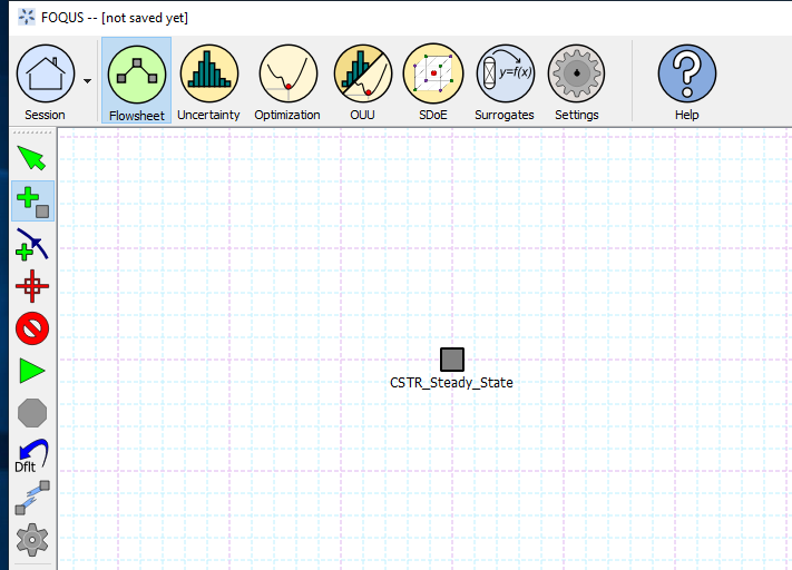
Figure 2 - Flowsheet Setup
Step 2: Define all input and output variables of the model as described in Figures 3 and 4.
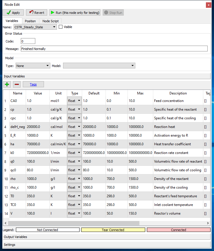
Figure 3 - Input Variables
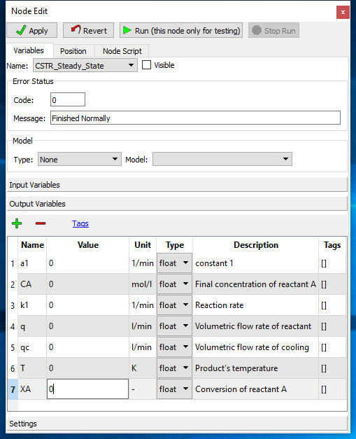
Figure 4 - Output Variables
Step 3: Create a MATLAB function solving the non-linear system of equations presented above. The MATLAB
function file (along with the FOQUS file for this example) can be found in the folder: examples/tutorial_files/MATLAB-FOQUS/Tutorial_1
Note
The examples/ directory refers to the location where the FOQUS examples were installed, as described in Install FOQUS Examples.
Step 4: Load FOQUS plugin named “matlab_fs” in the simulation node as shown Figure 5. In the node editor, under “Type” option, choose “plugin”, and under “Model” option choose “matlab_fs”.
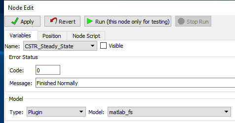
Figure 5 - FOQUS plugin for MATLAB-FOQUS interface
Step 5: In the Node Script tab write the code as shown in Figure 6.
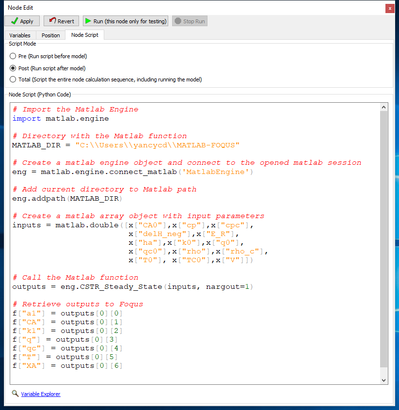
Figure 6 - Node Script Code
Note
The code shown in Figure 6 is intended to: 1) connect to the current MATLAB session, 2) create a MATLAB array object containing the input parameters for the MATLAB model, 3) Call the MATLAB function/model, and 4) Retrieve the outputs from the MATLAB function to FOQUS output variables.
The code is below:
 1
 2
 3
 4
 5
 6
 7
 8
 9
10
11
12
13
14
15
16
17
18
19
20
21
22
23
24
25
26
27
28
29
30
# Import the Matlab Engine
import matlab.engine

# Directory with the Matlab function
MATLAB_DIR = "C:\\Users\\yancycd\\MATLAB-FOQUS"

# Create a matlab engine object and connect to the opened matlab session
eng = matlab.engine.connect_matlab('MatlabEngine')

# Add current directory to Matlab path
eng.addpath(MATLAB_DIR)

# Create a matlab array object with input parameters
inputs = matlab.double([x["CA0"],x["cp"],x["cpc"],
         x["delH_neg"],x["E_R"],
         x["ha"],x["k0"],x["q0"],
         x["qc0"],x["rho"],x["rho_c"],
         x["T0"], x["TC0"],x["V"]])

# Call the Matlab function
outputs = eng.CSTR_Steady_State(inputs, nargout=1)

# Retrieve outputs to Foqus
f["a1"] = outputs[0][0]
f["CA"] = outputs[0][1]
f["k1"] = outputs[0][2]
f["q"] = outputs[0][3]
f["qc"] = outputs[0][4]
f["T"] = outputs[0][5]
f["XA"] = outputs[0][6]
Step 6: Run the node simulation to test if the simulation is working properly.
Step 7: Under the uncertainty tab in FOQUS, select Add New option to generate a new simulation ensemble. Select
Use Flowsheet option. Fix all variables except the volume, which will be a variable with bounds 50-150 l. Select
Latin Hypercube sampling method with 100 samples, and then generate the samples. Figure 7 represents the simulation
ensemble generation.
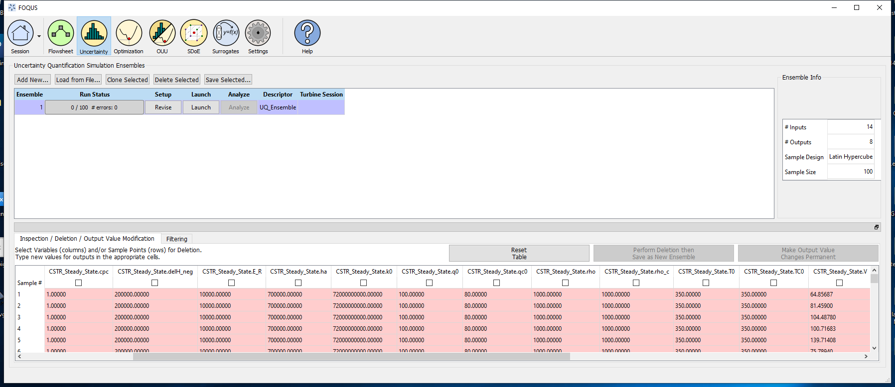
Figure 7 - Ensemble Generation
Step 8: Launch the simulations. Figure 8 represents the simulation results.
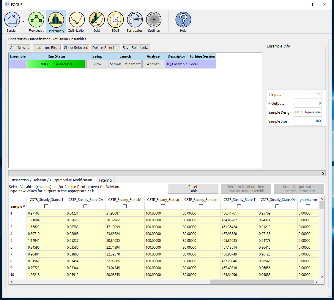
Figure 8 - Ensemble Results
Now, plotting the conversion vs the reactor’s volume, a similar figure to Figure 9 must be obtained.

Figure 9 - Conversion of Reactant A vs Reactor’s Volume
Tutorial 2: MATLAB script implementation
Step 1: Follow steps 1-3 from the Tutorial 1: MATLAB - FOQUS direct section. Users need to take care when defining the MATLAB function
for the model in step 3 as it is necessary to define the MATLAB function inputs in the same order as were defined in the FOQUS flowsheet.
Step 2: Follow step 6 from the Tutorial 1: MATLAB - FOQUS direct section to generate a new simulation ensemble.
Step 3: Select the new generated UQ_Ensemble and click on Save Selected to save the ensemble as a PSUADE file. Choose a folder to save the file
and name it as data.dat.
Step 4: Create a new MATLAB script to call the matlab_foqus_script.m file (which is distributed with FOQUS and can be found in examples/tutorial_files/MATLAB-FOQUS/Tutorial_2),
and pass to it the MATLAB function containing the model. Below is an example of the code that needs to be executed. In examples/tutorial_files/MATLAB-FOQUS/Tutorial_2
you can find a MATLAB file name example_2_matlab_foqus.m with the code, and you can simply execute it:
Note
After executing the code above, a new outputs.csv is created with the sample results from MATLAB. This is a file fully compatible with FOQUS.
Step 5: Under the uncertainty module, click on Load from File. Then choose .csv format file option and select the outputs.csv file created in
the previous step. A new window will ask you the number of inputs that contain the outputs.csv file (see Figure 10), for this example is 14.
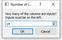
Figure 10 - Number of Inputs in the Outputs File
Step 6: Now, you have a new ensemble named “output.csv” with all input and outputs variables (see Figure 11), which can be used for other advanced analysis in the uncertainty module or any other FOQUS module.
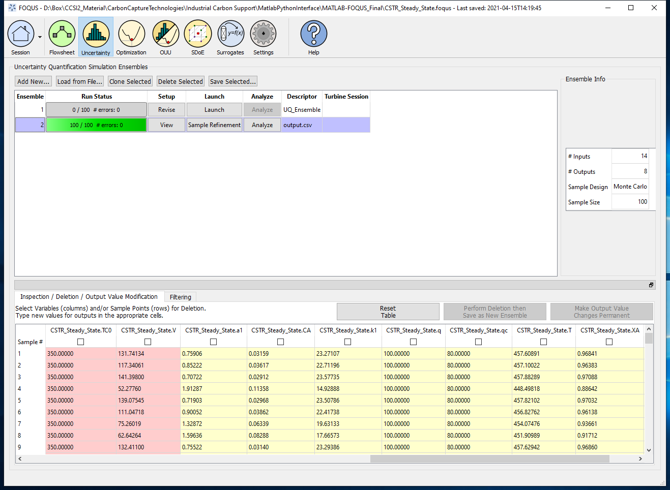
Figure 11 - New Ensemble with MATLAB Results
If you plot the conversion vs the reactor’s volume, you should get the Figure 9.